A wide range of complex systems can be effectively described as collections of point particles interacting through a combination of short- and long-range forces. This modelling paradigm has deep roots in classical many-body theory—such as gravitational dynamics, electron transport in semiconductors, and kinetic theory in statistical physics—and has recently gained significant traction in other scientific domains, including biology, social sciences, machine learning, and optimisation (see Carrillo et al. 2010, 2019g, 2022c, 2018a; Bailo et al. 2024). As a result, aggregation–diffusion modelling has become a vibrant and rapidly expanding area of research.
These models are remarkably versatile, spanning both microscopic and macroscopic scales. Applications include ion channel transport, chemotaxis, bacterial alignment, cellular adhesion, angiogenesis, animal group dynamics, and human crowd movement. In such systems, interactions between individuals are typically characterised by long-range attractive forces—arising from mechanisms such as ligand binding, electrical interactions, or social affinity—combined with short-range repulsive effects caused by physical constraints such as volume exclusion and crowding.
Various agent-based (microscopic) approaches have been developed to capture these dynamics, including cellular automata and driven Brownian particle models, all of which can encode rich and complex behaviour. However, rigorous analytical insight is most effectively achieved through the study of the mean-field limit (or related formulations), which describes the behaviour of the system as the number of interacting agents becomes large (see Oelschläger 1990a; Bolley et al. 2011; Jabin 2014).
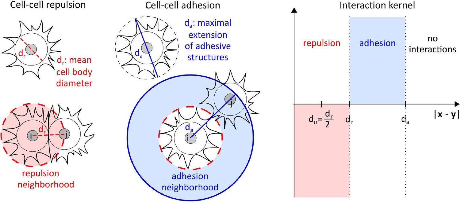
To illustrate this framework, consider a system composed of two distinct cell populations, each expressing different surface proteins or ligands (such as cadherins or nectins). Let the nuclei of the first cell type be located at positions {xi}i=1N\{x_i\}_{i=1}^N{xi}i=1N, and those of the second at {yj}j=1M\{y_j\}_{j=1}^M{yj}j=1M, with N=MN = MN=M for simplicity. Cells interact through medium-range attraction (e.g. via filopodia) and strong short-range repulsion due to size and volume constraints (see Fig. 1). Assuming that the interaction forces are radial and conservative, with interaction potentials WabNW^{N}_{ab}WabN for a,b=1,2a,b = 1,2a,b=1,2, the microscopic dynamics can be described by a system of coupled ordinary differential equations.
Under appropriate assumptions, the empirical measures associated with this agent-based model—defined as weighted sums of Dirac delta distributions at particle locations—converge, in the many-particle limit, to macroscopic, normalised cell density distributions ρ1(t,x)\rho_1(t,x)ρ1(t,x) and ρ2(t,x)\rho_2(t,x)ρ2(t,x). In biological settings, it is reasonable to assume that attractive interactions act only within a finite cut-off radius RRR, while repulsion is strictly localised (Calvez and Carrillo 2012). This motivates a natural scaling of the interaction potentials of the form WabN=εδ0+WabW^{N}_{ab} = \varepsilon \delta_0 + W_{ab}WabN=εδ0+Wab as N→∞N \to \inftyN→∞, where ε\varepsilonε represents the characteristic cell volume (Oelschläger 1990a; Carrillo et al. 2019g).
In this limit, the system converges to a coupled mean-field aggregation–diffusion model for the cell densities. More generally, such systems can be cast in the form of a continuum transport equation
∂tρ+∇⋅(ρu)=0,u=−∇ξ,ξ=U(ρ)+V+W∗ρ,\partial_t \rho + \nabla \cdot (\rho u) = 0, \quad u = -\nabla \xi, \quad \xi = U(\rho) + V + W * \rho,∂tρ+∇⋅(ρu)=0,u=−∇ξ,ξ=U(ρ)+V+W∗ρ,
which governs the kinematic evolution of a population density ρ(t,x)\rho(t,x)ρ(t,x). Here, the velocity field results from the interplay of three mechanisms: diffusion driven by local repulsion or stochastic effects (modelled by a convex function U(ρ)U(\rho)U(ρ)), drift induced by an external potential V(x)V(x)V(x), and nonlocal interactions represented by a symmetric interaction potential W(x)=W(−x)W(x) = W(-x)W(x)=W(−x) (see Bodnar and Velazquez 2006; Topaz et al. 2006).
Common choices for the diffusion term include linear diffusion U(s)=slogsU(s) = s \log sU(s)=slogs and nonlinear diffusion U(s)=sm/(m−1)U(s) = s^m/(m-1)U(s)=sm/(m−1) for m>0m > 0m>0 (Vázquez 2007). In the porous medium regime (m>1m > 1m>1), diffusion is stronger in regions of high density, while in the fast diffusion regime (m<1m < 1m<1), it is enhanced in low-density regions. Confining potentials of the form V(x)=∣x∣pV(x) = |x|^pV(x)=∣x∣p, with p>0p > 0p>0, frequently arise in Fokker–Planck and McKean–Vlasov equations (Carrillo et al. 2003, 2020b, 2022b).
Citation:
TY - CHAP
AU - Bailo, Rafael
AU - Carrillo, J.A
AU - Gómez-Castro, David
PY - 2026/01/12
SP - 177
EP - 200
SN - 978-981-95-1445-8
T1 - Aggregation-Diffusion Equations for Collective Behaviour in the Sciences
VL -
DO - 10.1007/978-981-95-1446-5_9
ER -
For full paper:
https://www.researchgate.net/publication/399682810_Aggregation-Diffusion_Equations_for_Collective_Behaviour_in_the_Sciences